ACTIVITY 6: Properties and Applications of the 2D Fourier Transform
-Jessica Nasayao
In this activity, our aim is to investigate the different properties of the Fourier transforms of different patterns and try to apply them to real world applications.
From the previous experiments, we were able to observe that the FT of a pattern inverts the pattern’s dimensions; e.g., what is narrow in the image’s axis will appear wide in it’s Fourier Transform, and vice versa. This property is called anamorphism. To demonstrate this property further, we applied FT to different patterns namely: a tall rectangle, a wide rectangle, and to two dots with varying spaces in between. The results are shown in the images below.
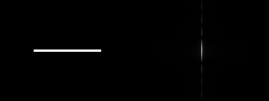
Figure 1. a) Wide rectangular pattern and b) its Fourier Transform
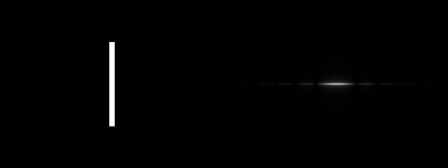
Figure 2 a) Tall rectangular pattern and b) its Fourier Transform
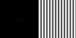
Figure 3 a) Two dots of relatively close spacing and b) its Fourier Transform
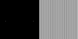
Figure 4 a) Two dots of relatively far spacing and b) its Fourier Transform
We can see that the bright bands of the tall rectangle’s Fourier transform lies along the x-axis, while those of the wide rectangle are on the y-axis. Taking the Fourier Transform of two bright dots placed closely together results in a corrugated roof of a small frequency. On the other hand, if placed far apart, the same bright dots will give a corrugated roof of a larger frequency.
Next, we want to know how rotating the patterns affects the Fourier transform. First, we get the Fourier Transform of a corrugated roof, as shown below.
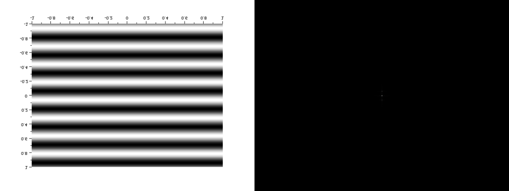
Figure 5 a) Corrugated roof of frequency 4 and b) its Fourier transform
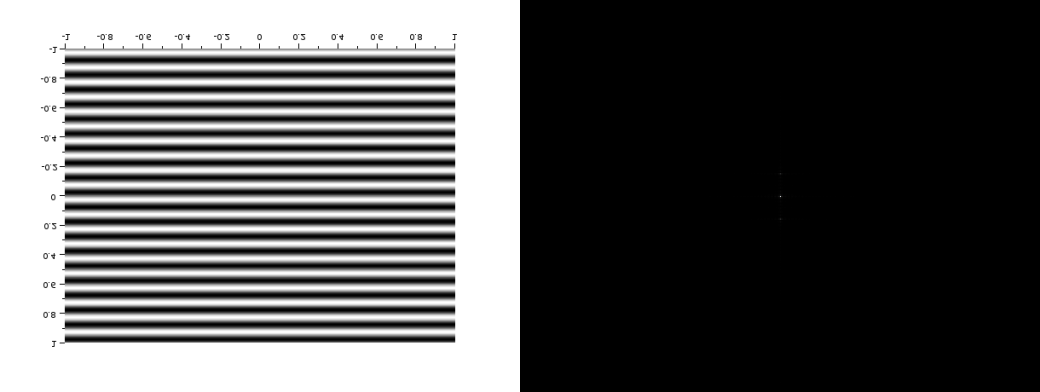
Figure 6 a) Corrugated roof of frequency 10 and b) its Fourier transform
We can see that as the frequency increases, the dots in the Fourier tranform gets further away from each other.
If we rotate the corrugated roof, the Fourier transform pattern also rotates, as shown in the images below:
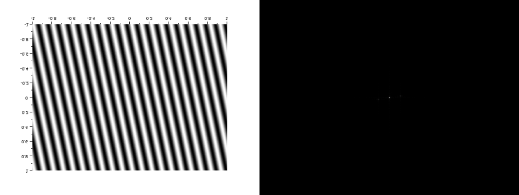
Figure 7 a) Corrugated roof rotated 30 degrees and b) its Fourier transform
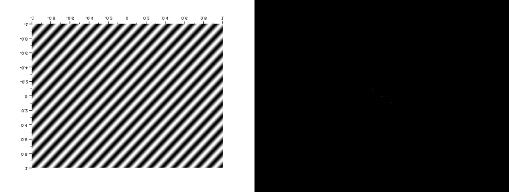
Figure 8 a) Corrugated roof rotated 120 degrees and b) its Fourier transform
If we try to synthesize a combination of sinusoids along the X and Y axes, the Fourier transform is also the combination of the individual Fourier transforms of the sinusoid, as shown in Figure 9.
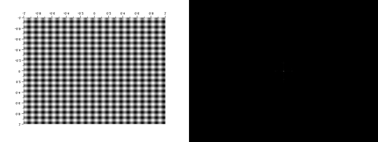
Figure 9. a) Mix of corrugated roofs running along the X and Y axes and b) its Fourier Transform
If we add a rotated sinusoid to this synthetic pattern, the Fourier will also be the combination of the Fourier transforms of the three sinusoids. The image of the Fourier Transform is slightly blurry though, but if you look closely, you can make out the pattern.
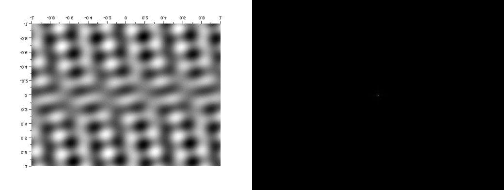
Figure 10. a) Mix of sinusoids of different orientations b)its Fourier Transform
Earlier, we displayed the Fourier transform of two dots along the x-axis, symmetric about the center. We also tried this on different patterns: two circles, two squares, and two Gaussians, and observed the results.
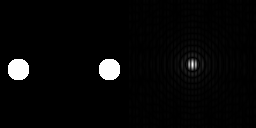
Figure 11. Fourier transform of two circles.
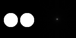
Figure 12. Fourier transform of two circles with a different radius.
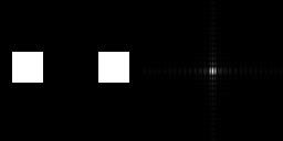
Figure 13. Fourier transform of two squares.
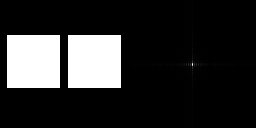
Figure 14. Fourier transform of squares of a different size.
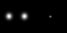
Figure 15. Fourier transform of two gaussians.
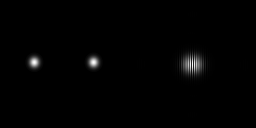
Figure 16. Fourier Tranform of two gaussians. (difference variance)
Now, what do you think will happen if we convolute a pattern to an image with randomly-positioned approximations of n dirac deltas? Turns out, the pattern will be repeated n times, each of themcentered on the dirac delta approximations, like the image below.
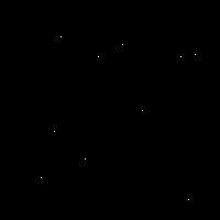
Figure 17. Dirac delta approximations.

Figure 18. Convolution with a small triangular pattern.
If we create an array of equally spaced dots along the x and y axes and take it’s Fourier transform, the result will look like the ones shown in the images below.
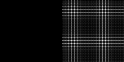
Figure 19. a) Equally spaced dots along the x and y axes b) its Fourier Transform
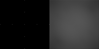
FIgure 20. a) Dots of different spacing b) its Fourier Transform
Now that we have already familiarized ourselves with the properties of Fourier transform, let’s try to use them in some real-world application. Consider, for example, this image of the moon:
Figure 21. Picture of the moon.
If we take the Fourier transform of that image, we get the following result:
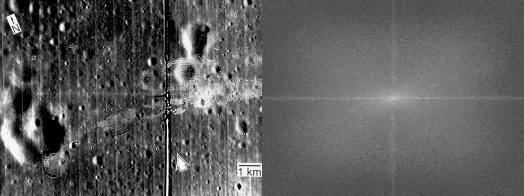
Figure 22. a) Grayscale of the image and b) its Fourier Transform
What we want to do is to try and see if we can remove the vertical and horizontal lines from the image. From the anamorphism property demonstrated earlier, we know that the horizonatal lines correspond to the vertical ones in the Fourier transform, and vice versa. We can try and make a mask such that these frequencies will be eliminated from our FT image and use inverse Fourier to revert back to the original image. The mask I used is shown below.
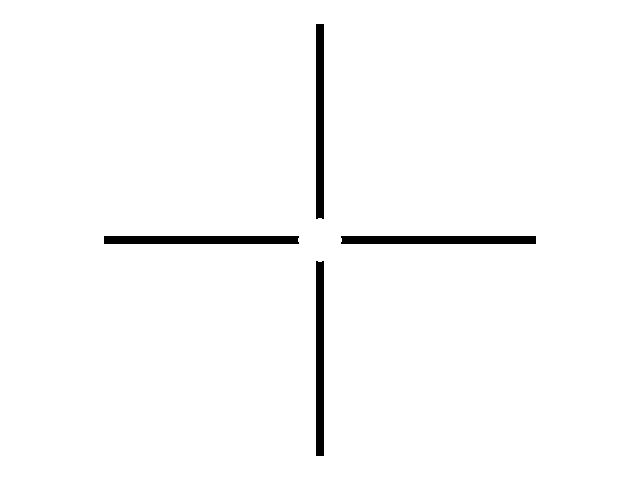
Figure 23. Mask used to eliminate vertical and horizontal lines in the image.
I convoluted this mask to the Fourier transform of my image and did an inverse fourier transform on the resulting matrix. The comparison between the original and the resulting image was shown below. The lines were visibly eliminated from the image.
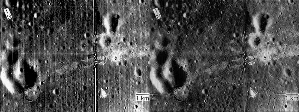
Figure 24. Comparison between the a) Original image and the b) result of the process.
We can apply the same logic to different images. Next, consider a scanned image of a fingerprint, shown below.
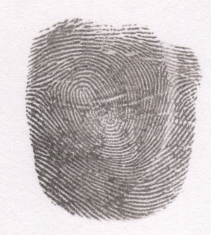
Figure 25. Scanned finger print. Image retrieved from: http://grupocasacam.com/covao/latent-fingerprints&page=5
Applying Fourier transformation to the image, we get:
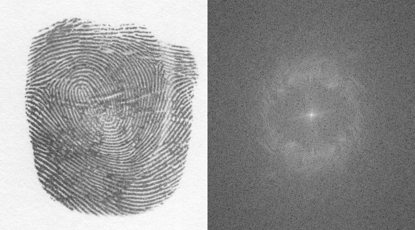
Figure 26. a) Grayscale of the fingerprint and the b) Log of its Fourier transform.
To eliminate the dark smudges of ink and hopefully enhance the ridges of our fingerprint, we use a mask that is produced by setting a threshold value on our FT image. The mask I used was shown below.
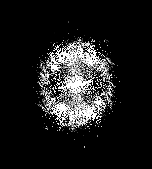
Figure 27. Mask used for ridge detection.
We now again apply the same process we did earlier and convolute this mask to the FT of our image. Shown below is the resulting image and its comparison to the original image after performing an inverse transform to the convoluted matrix. The blotches between ridges are visibly reduced and the ridges enhanced.
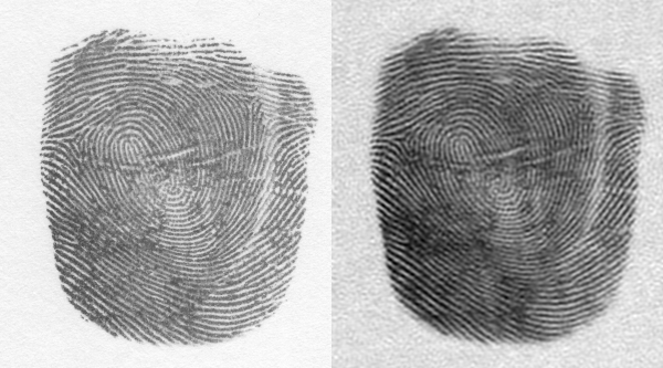
Figure 28. Image of the fingerprint a)Before ridge detection and processing and b) after processing.
Self-score: 10/12
